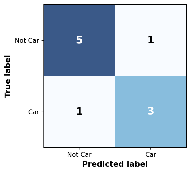
Ultralytics YOLO Foundations: Part 4

Evaluation & Deployment

2026-03-13

7. Model Evaluation

How good is your model?

Binary Classification Basics

When evaluating models, every prediction falls into one of four categories. Let’s use detecting a “Car” as an example:

  • True Positive (TP): Model correctly predicted “Car” and there is a car there.
  • False Positive (FP): Model predicted “Car”, but there was no car there (False Alarm).
  • True Negative (TN): Model correctly predicted “Not Car” for background.
  • False Negative (FN): There is a car in the image, but the model missed it.

The Confusion Matrix

Accuracy : 0.80
Precision: 0.75
Recall   : 0.75


Matrix Layout:

  • Rows: True Labels (Actual)
  • Columns: Predicted Labels
  • Diagonal: Correct predictions (TP & TN)
  • Off-Diagonal: Errors (FP & FN)

The Problem with Accuracy

The most intuitive metric is Accuracy (Total Correct / Total Predictions). But is it enough?

Imagine a dataset with 1 “Car” and 99 “Not Car” (background) images. If a model simply predicts “Not Car” for everything:

  • TP = 0, FN = 1 (Missed the only car)
  • TN = 99, FP = 0

\[Accuracy = \frac{0 + 99}{100} = 99\%\]

It achieved 99% Accuracy despite being completely useless at finding cars!

This is the Class Imbalance Problem, common in object detection where most of an image is empty background.

Precision, Recall, and F1

To solve the Class Imbalance Problem, we focus on metrics that ignore True Negatives:

  • Precision: When it guesses an object, is it correct? (Quality) \[Precision = \frac{TP}{TP + FP}\]
  • Recall: Out of all actual objects, how many did it find? (Quantity) \[Recall = \frac{TP}{TP + FN}\]
  • F1-Score: The harmonic mean of Precision and Recall. \[F_1 = 2 \times \frac{Precision \times Recall}{Precision + Recall}\]

Interactive Demo: Threshold Trade-off

The Confidence Threshold Trade-off

The Confidence Threshold dictates how “sure” the model must be to output a prediction. Adjusting it directly affects your balance of errors:

  • High Threshold (e.g., 0.80): The model is strict.
    • Decreases False Positives (FP) (fewer false alarms \(\rightarrow\) Higher Precision)
    • Increases False Negatives (FN) (misses more objects \(\rightarrow\) Lower Recall)
  • Low Threshold (e.g., 0.20): The model is loose.
    • Increases False Positives (FP) (more false alarms \(\rightarrow\) Lower Precision)
    • Decreases False Negatives (FN) (catches almost everything \(\rightarrow\) Higher Recall)

The PR Curve & Average Precision (AP)


Step 1: Gather We take every “Car” prediction the model made across the whole test set.


Step 2: Sort We sort them from highest confidence (e.g., \(0.99\)) to lowest (e.g., \(0.10\)).


Step 3: Calculate We calculate Precision and Recall at every single step of that sorted list.


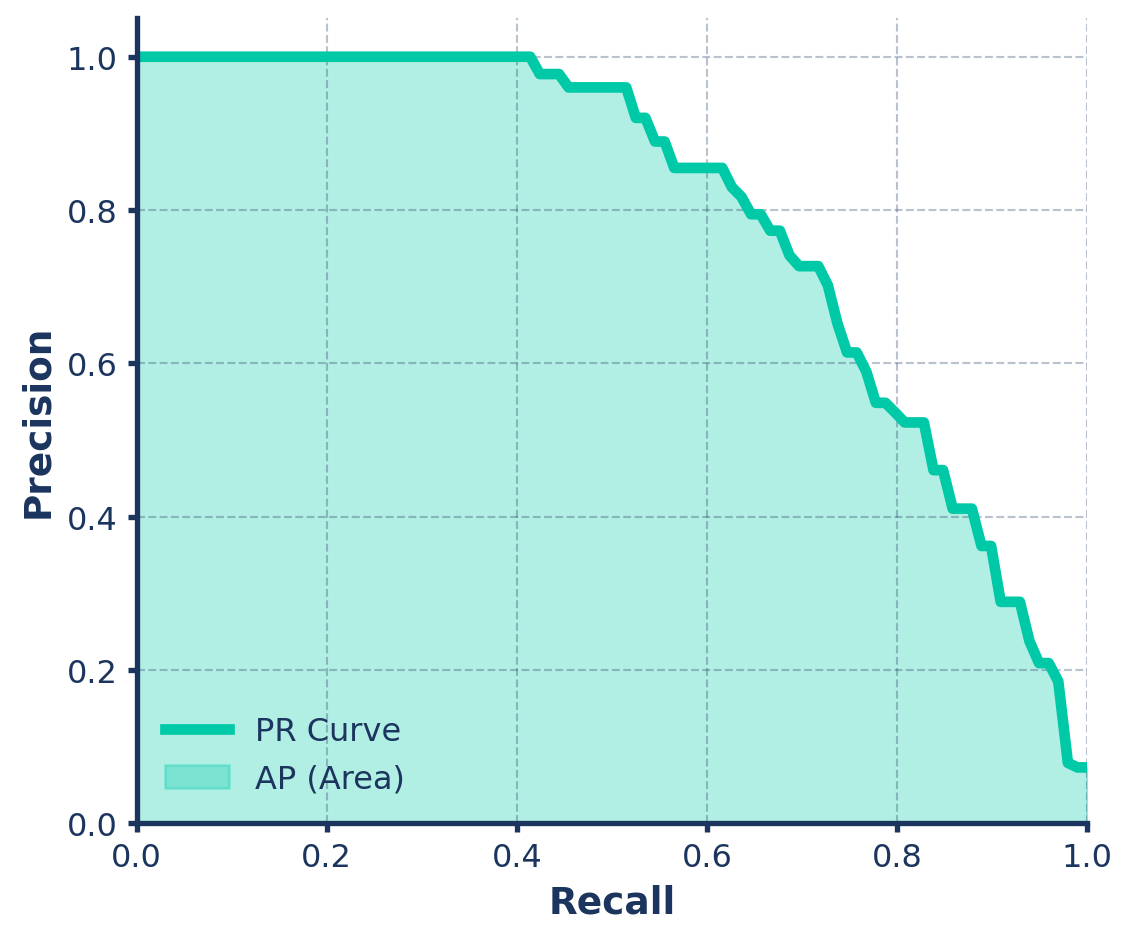
Average Precision (AP) is simply the area under this Precision-Recall (PR) curve!

Intersection over Union (IoU)

How perfectly does the predicted bounding box overlap the ground truth box?

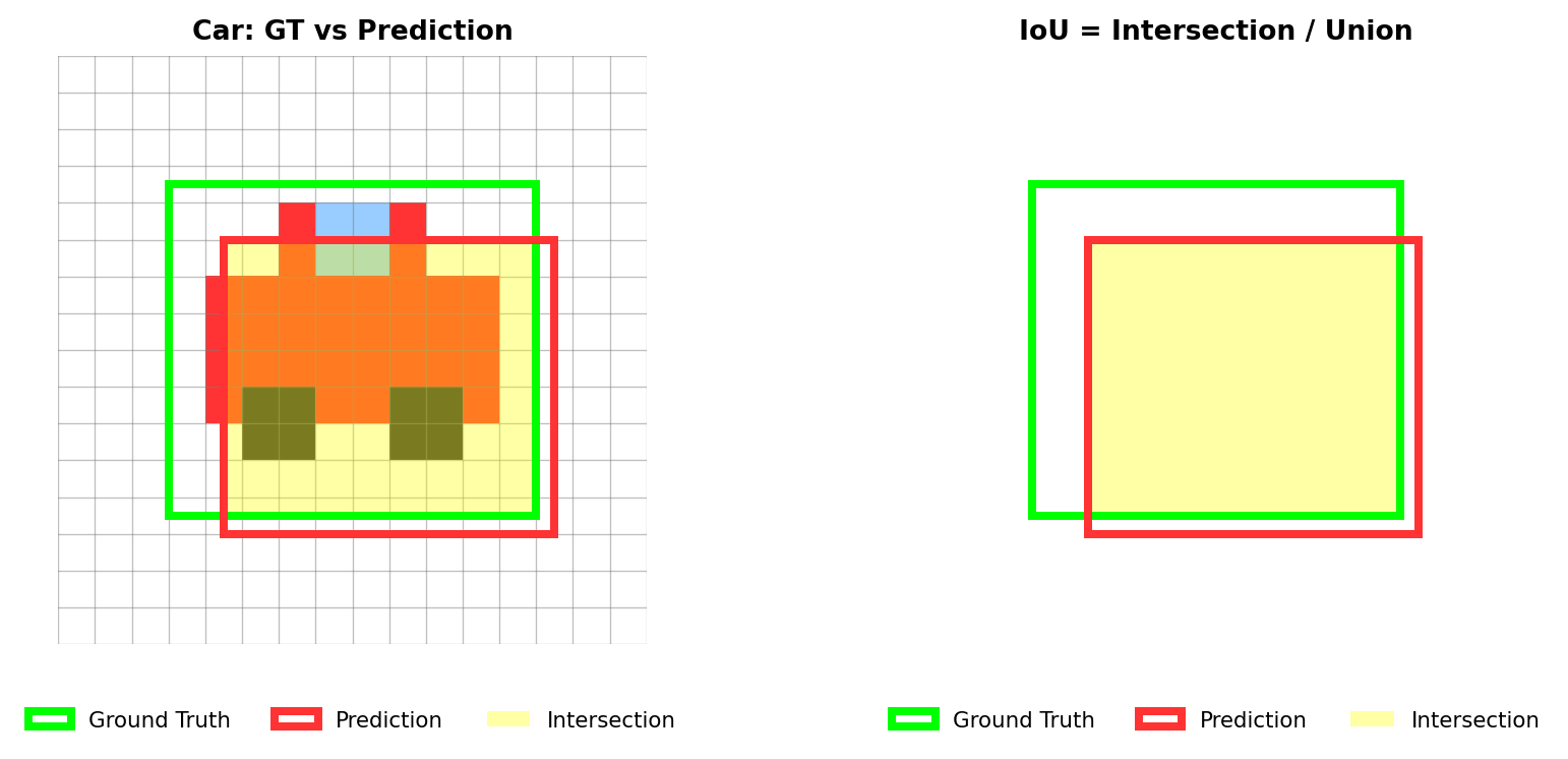
Rule of Thumb: A prediction is typically considered a “True Positive” (correct) if the IoU is > 0.50.

The “Double Penalty” of IoU

A prediction must be accurate in location (\(IoU \ge 0.5\)) to count as a True Positive (TP).

What happens if a prediction misses (\(IoU < 0.5\))?

Important

It hurts your evaluation twice!

  • False Positive (FP): The poorly placed prediction is a “False Alarm”.
  • False Negative (FN): The real object is considered “Missed”.

The Car Example: You draw a bad box for a car (IoU < 0.5).

  • FP: You generated a useless box (false alarm penalty).
  • FN: The actual car was never successfully claimed (missed target penalty).

Handling Multiple Detections

A common question is: “What if the model predicts multiple boxes for the exact same object?”

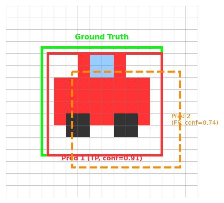
Rule: One Ground Truth = Only One TP

  1. The Winner: Highest IoU (Pred 1) becomes the True Positive (TP).
  2. The Duplicate: Extra boxes (Pred 2) become False Positives (FP).

Mean Average Precision (mAP)

Once we have the AP for every class (Cars, Pedestrians, Trees, etc.), we simply take the arithmetic mean.

\[mAP = \frac{AP_{cars} + AP_{pedestrians} + AP_{trees} + ...}{Total\ Number\ of\ Classes}\]

  • mAP50: Accuracy considering only “easy” detections (IoU > 0.50).
  • mAP50-95: The strict evaluation averaged across multiple IoU thresholds (from 0.50 to 0.95).

Validating the Model (YOLO CLI/Python)

We use the val mode to evaluate a trained model. YOLO automatically generates graphs (confusion_matrix.png, PR_curve.png) in your runs/detect/val folder.

yolo val model=best.pt data=data.yaml
from ultralytics import YOLO

model = YOLO("best.pt")
metrics = model.val(data="data.yaml")

Docs Reference: Model Evaluation Insights

8. Deployment

Taking it to production.

Exporting Models

A PyTorch .pt file is great for research, but slow in production. Convert to optimized formats using the export mode!

# Export to ONNX (Great for CPU)
yolo export model=best.pt format=onnx

# Export to OpenVINO (Intel) or TensorRT (Nvidia GPUs)
yolo export model=best.pt format=openvino
from ultralytics import YOLO

model = YOLO("best.pt")
model.export(format="onnx")
model.export(format="openvino")

Docs Reference: Export

Inference with Exported Models

You don’t need complex deployment code to use your exported models. The Ultralytics API loads them just like a standard PyTorch .pt file!

yolo predict model=best.onnx source="https://ultralytics.com/images/bus.jpg"
from ultralytics import YOLO

model = YOLO("best.onnx")
results = model.predict(source="https://ultralytics.com/images/bus.jpg")
print(results[0].boxes) 

Docs Reference: Predict with Exported Models

Conclusion

Course Wrap-up

The Ultralytics Ecosystem

You have learned:

  • Tasks: Object Detection, Segmentation, Pose Estimation, and OBB.
  • Solutions: Effortlessly integrating advanced logic out-of-the-box.
  • Datasets: Structuring arrays and labels for different tasks.
  • Tools: Navigating the CLI, YAML configs, and hyperparameters.
  • Evaluation: Interpreting metrics, confidence thresholds, and PR curves.
  • Deployment: Exporting PyTorch models for production speed.

What’s Next?

Your Turn!

Apply these foundational skills to solve real-world problems. Whether building smart security cameras, medical imaging tools, or autonomous vehicles, the core principles remain the same.

Q&A

Thank You!

Any questions?