graph TD
Q["New Query"] --> E["Embed Query\n(sentence-transformers)"]
E --> S["Cosine Similarity Search\nvs cache entries"]
S -->|sim > 0.93| HIT["Cache HIT\nReturn stored response"]
S -->|sim ≤ 0.93| MISS["Cache MISS"]
MISS --> LLM["Call LLM API"]
LLM --> STORE["Store response + embedding\nin cache"]
STORE --> RESP["Return response"]
HIT --> RESP
style HIT fill:#00C9A7,stroke:#1C355E,color:#1C355E
style MISS fill:#FF7A5C,stroke:#1C355E,color:#1C355E
style LLM fill:#9B8EC0,stroke:#1C355E,color:#1C355E
Production Optimization
RAG Foundations & Data Pipelines — Session 6
2026-04-26
A. Prototype to Production
Scaling your RAG system for real users
Agenda
- A. Prototype to Production — The three optimization axes
- B. HNSW Benchmarking — Systematic parameter tuning
- C. Quantization — Trading precision for massive scale
- D. Caching Strategies — Semantic and Response caching
- E. Zero-Downtime Reindexing — Production update strategies
- F. Cost Planning — Budgeting for vector infrastructure
- G. Final Architecture — The complete Research Assistant
The Scale Question
From Prototype to Product
Your RAG system works on 1,000 documents. But production means:
- 100K+ documents growing 10% monthly
- Thousands of queries/day with p95 < 5 seconds
- Zero downtime during knowledge base updates
- Budget approval with a clear cost forecast
Three Optimization Axes
Speed
- HNSW parameter tuning
ef_searchoptimization- Query caching
- Batch operations
Target: < 50ms per search
Accuracy
Mandef_construction- Quantization impact
- Recall@10 monitoring
- Re-ranking quality
Target: > 0.95 Recall@10
Cost
- Memory footprint
- Storage per vector
- API call pricing
- Managed vs self-hosted
Target: < $0.10 per query (including LLM)
B. HNSW Benchmarking
Systematic parameter tuning
Benchmarking Framework
def build_and_benchmark_hnsw(embeddings,
    M_list=[16, 32, 64],
    ef_construction_list=[100, 200, 400],
    ef_search_list=[50, 100, 200]):
    """Benchmark HNSW configurations."""

    d = embeddings.shape[1]  # embedding dimension
    results = []

    for M in M_list:
        for ef_con in ef_construction_list:
            index = faiss.IndexHNSWFlat(d, M)
            index.hnsw.efConstruction = ef_con
            index.add(embeddings)

            for ef_search in ef_search_list:
                index.hnsw.efSearch = ef_search
                # Benchmark: time + recall
                ...
                results.append({
                    'M': M, 'ef_con': ef_con,
                    'ef_search': ef_search,
                    'search_ms': avg_ms,
                    'recall': recall_at_10})
    return results
Parameter Grid
| Parameter | Values Tested | Effect |
|---|---|---|
| M | 16, 32, 64 | Graph connectivity (memory) |
| ef_construction | 100, 200, 400 | Index build quality (build time) |
| ef_search | 50, 100, 200 | Query-time search depth (latency) |
Total configurations: 3 x 3 x 3 = 27 experiments
Search Time vs Recall
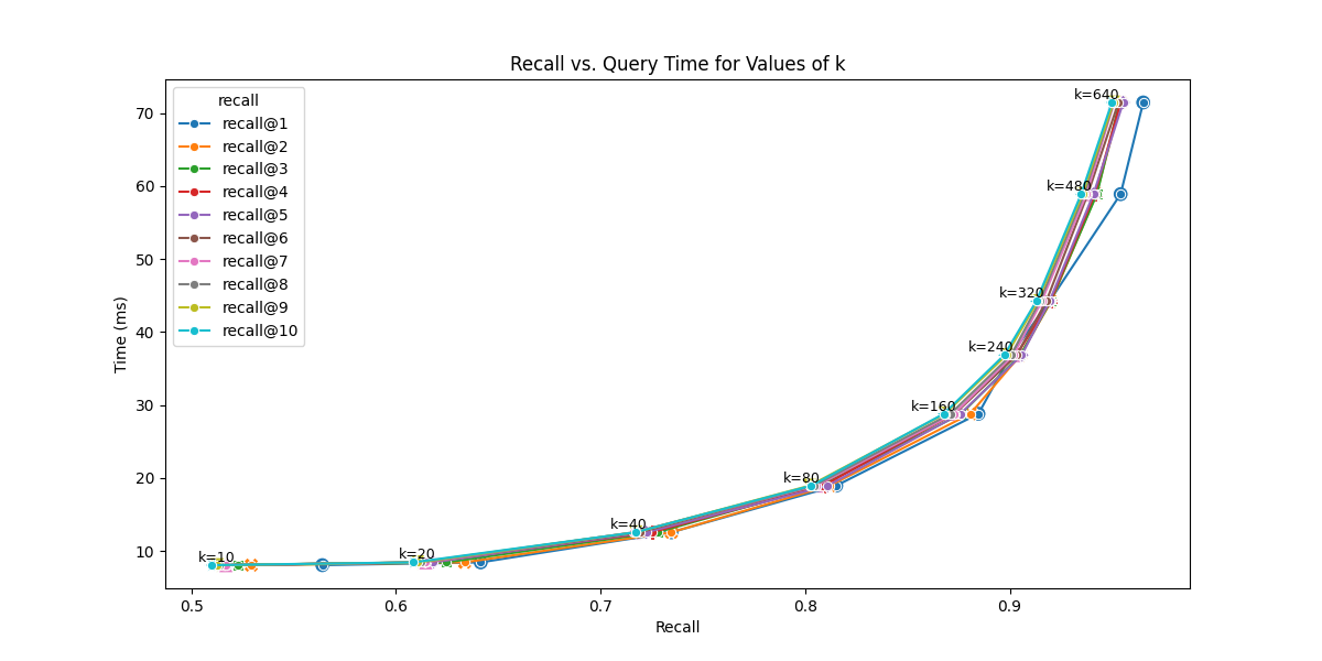
SOURCE: OpenSource Connections (2025). The Pareto frontier shows the optimal speed-accuracy trade-offs for HNSW.
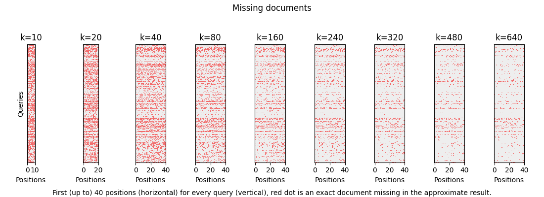
SOURCE: OpenSource Connections (2025). Diagnostic visualization showing “missing documents” (red dots) at different search depths (k or ef_search), proving how recall improves as search depth increases.
Starting Points
Rules of Thumb
| Dataset Size | M | ef_construction | ef_search |
|---|---|---|---|
| < 100K vectors | 16 | 200 | 50-100 |
| 100K - 1M | 32 | 200 | 100-200 |
| > 1M | 32-64 | 400 | 200+ |
You can increase
ef_searchat query time without rebuilding the index. Start low, increase until latency budget is exhausted.
C. Quantization
Trading precision for massive scale
Why Quantize?
100M vectors × 1536 dimensions × 4 bytes = ~614 GB (or ~572 GiB) just for the vectors.
Quantization reduces vector size by storing with lower precision:
- Full float32: 4 bytes/dimension → 6 KB per vector
- SQ8 (8-bit int): 1 byte/dimension → 1.5 KB per vector
- Binary: 1 bit/dimension → 192 bytes per vector
At 100M vectors, going from float32 to SQ8 saves ~460 GB (~430 GiB) of memory.
Quantization Types
| Type | Compression | Recall Impact | Speed Impact |
|---|---|---|---|
| Scalar (SQ8) | 4x | Minimal (~2%) | Faster (cache-friendly) |
| Product (PQ) | 10-100x | Moderate (~5-15%) | Much faster |
| Binary | 32x | Variable (~5-15%) | Fastest |
Recall impact figures are approximate and vary significantly with dataset size, index parameters, and embedding model. Always validate against your evaluation suite.
FAISS Indexes
# 1. Flat Index (Exact - Baseline)
index_flat = faiss.IndexFlatL2(d)

# 2. HNSW (Approximate, Full Precision)
index_hnsw = faiss.IndexHNSWFlat(d, M=32)

# 3. Scalar Quantization (SQ8)
index_sq8 = faiss.IndexScalarQuantizer(
    d, faiss.ScalarQuantizer.QT_8bit)
index_sq8.train(embeddings)

# 4. IVF + Product Quantization (IVFPQ)
quantizer = faiss.IndexFlatL2(d)
index_ivfpq = faiss.IndexIVFPQ(
    quantizer, d, nlist=1024, m=96, nbits=8)
index_ivfpq.train(embeddings)
Speed / Accuracy / Memory
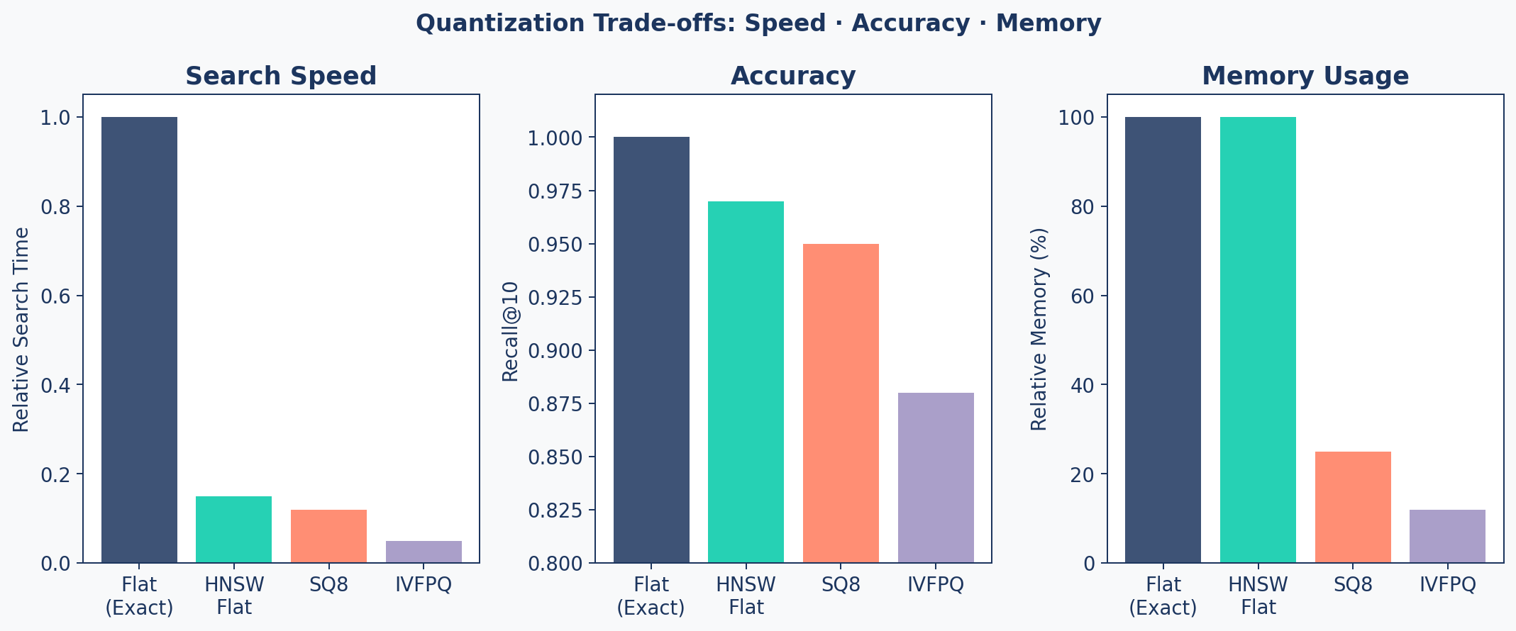
When to Use What
| Scale | Recommended Index | Why |
|---|---|---|
| < 100K | HNSW Flat | Best accuracy, memory is fine |
| 100K - 1M | HNSW + SQ8 | 4x memory savings, minimal recall loss |
| 1M - 10M | IVF + PQ | Major memory savings, fast search |
| > 10M | IVF + PQ + OPQ | Maximum compression needed |
Always A/B Test
Quantization must be validated against your ground truth metrics from the evaluation suite. Never assume recall is “good enough” — measure it.
D. Caching Strategies
Embedding-based similarity matching to skip redundant LLM calls
Response Caching
During development and production, you often see the exact same queries repeated.
LiteLLM ships with built-in exact-match caching — one line to enable it globally:
Limitation: Exact match fails if the user adds a single space or changes capitalization.
What is Semantic Caching?
The Key Insight
Two queries can be semantically identical but lexically different: "What is the capital of France?" and "Tell me France's capital city" should return the same cached answer.
How it works:
- Embed the incoming query → vector
- Search cache for similar vectors (cosine similarity)
- If similarity > threshold (e.g., 0.93) → return cached response
- Otherwise → call LLM, store result + embedding in cache
Semantic Cache Flow
Cost Impact of Caching
| Scenario | Daily Requests | Cache Hit Rate | Daily Cost | Notes |
|---|---|---|---|---|
| No cache | 10,000 | 0% | $150 | Baseline |
| Weak cache (sim > 0.99) | 10,000 | 15% | $127.50 | Conservative, high precision |
| Strong cache (sim > 0.93) | 10,000 | 30% | $105 | … |
| Aggressive (sim > 0.90) | 10,000 | 45% | $82.50 | Risk of semantic mismatches |
Threshold Trade-off
Lower threshold → more hits, but risk of semantically different queries getting wrong answers.
E. Zero-Downtime Reindexing
Updating production without breaking it
Two Strategies
Incremental Updates
- Upsert new documents
- Index is not re-optimized
- Works for small, regular additions
- Quality can degrade over time
Alias-Switching (Full Reindex)
- Build a brand new index
- Backfill all data
- Swap pointer atomically
- Delete old index
Zero-downtime, always optimal
Alias-Switching
sequenceDiagram
    participant App as Application
    participant Old as Index v1 (Live)
    participant New as Index v2 (Building)
    participant Alias as Alias Config

    App->>Alias: Read: "live = v1"
    App->>Old: Serve queries
    Note over New: Build new index<br/>Backfill all data
    New->>New: Verify data integrity
    App->>Alias: Write: "live = v2"
    App->>New: Serve queries (instant switch)
    Note over Old: Delete after cooldown
Code: PineconeReindexer
class PineconeReindexer:
    def execute_zero_downtime_update(self, chunks):
        # 1. Generate unique name
        timestamp = datetime.utcnow().strftime("%Y%m%d%H%M")
        new_name = f"research-assistant-{timestamp}"

        # 2. Create & Populate new index
        self.create_index(new_name)
        self.backfill_data(new_name, chunks)

        # 3. Get current live index
        old_name = self.alias_manager.get_live_index()

        # 4. ATOMIC SWITCH
        self.alias_manager.set_live_index(new_name)

        # 5. Cleanup old index (after cooldown)
        if old_name and old_name != new_name:
            self.pc.delete_index(old_name)
Safety Checklist
Before Switching Live
- New index has same or more documents than old
- Spot-check 10 known queries produce correct results
- Eval metrics (Hit Rate, MRR) meet thresholds
- Rollback plan — keep old index for 24h before deletion
- Test on staging first — never go straight to production
F. Cost Planning
Budgeting for vector infrastructure
Cost Formula
def estimate_monthly_cost(config, num_vectors,
                          reads_per_month, writes_per_month):
    # Vector storage
    bytes_per_vector = config.dimension * 4  # float32
    storage_gb = (num_vectors * bytes_per_vector) / 1e9

    # Metadata storage
    meta_gb = (num_vectors * config.meta_bytes) / 1e9

    # Total cost
    storage_cost = (storage_gb + meta_gb) * config.$/gb
    read_cost = (reads_per_month / 1e6) * config.$/M_reads
    write_cost = (writes_per_month / 1e6) * config.$/M_writes

    return config.base_fee + storage_cost + read_cost + write_cost
Cost Forecast
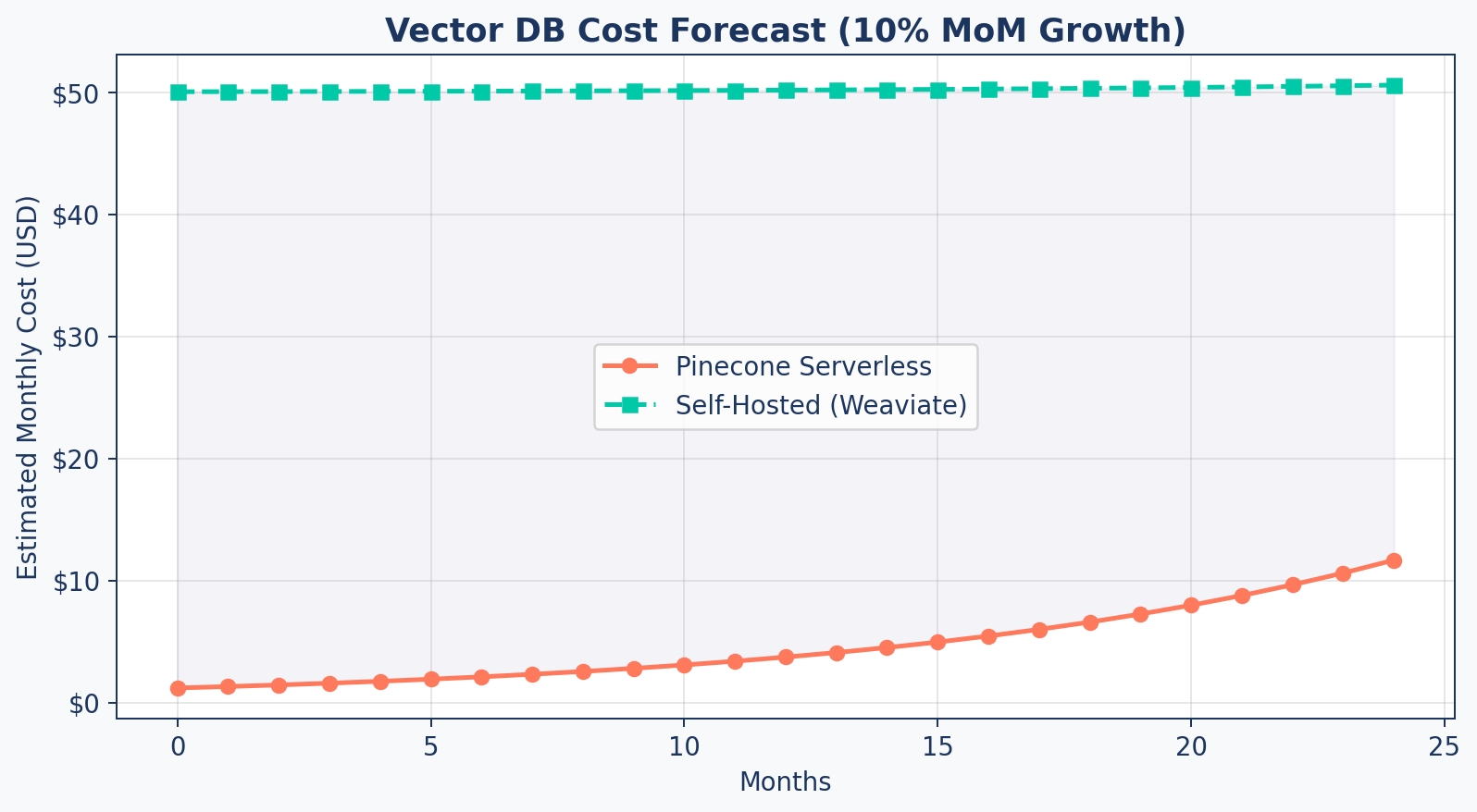
Reduction Strategies
| Strategy | Savings | Trade-off |
|---|---|---|
| Quantization (SQ8) | 75% storage | Small recall loss |
| Larger chunks | Fewer vectors | Less precision |
| Metadata pruning | Up to 50% metadata storage | Less filtering capability |
| Tiered storage | 50%+ | Cold data has higher latency |
| Caching | Varies by query distribution | Stale results for rare queries |
G. Final Architecture
The Research Assistant Picture
A System Architecture
flowchart LR
    User["User Query"] --> QP["Query Processor"]
    QP -->|"Expanded Queries"| AR["Advanced Retriever"]
    AR -->|"Hybrid Search"| VS[("Vector Store")]
    AR -->|"BM25 Search"| KS[("Keyword Index")]
    VS & KS --> Cands["Candidate Pool"]
    Cands --> RR["Cross-Encoder<br/>Re-ranker"]
    RR -->|"Top K"| CM["Context Manager"]
    CM -->|"Pruned Context"| Gen["LLM Generation"]
    Gen -->|"Answer + Citations"| User

    subgraph Offline Pipeline
        Ingest["Ingestion"] --> VS
        Eval["DeepEval Suite"] -.->|"Grades"| Gen
    end

    style User fill:#9B8EC0,stroke:#1C355E,color:#fff
    style QP fill:#9B8EC0,stroke:#1C355E,color:#fff
    style AR fill:#00C9A7,stroke:#1C355E,color:#fff
    style VS fill:#1C355E,stroke:#1C355E,color:#fff
    style KS fill:#1C355E,stroke:#1C355E,color:#fff
    style RR fill:#FF7A5C,stroke:#1C355E,color:#fff
    style CM fill:#FF7A5C,stroke:#1C355E,color:#fff
    style Gen fill:#FF7A5C,stroke:#1C355E,color:#fff
    style Ingest fill:#00C9A7,stroke:#1C355E,color:#fff
    style Eval fill:#9B8EC0,stroke:#1C355E,color:#fff
ResearchAssistantService
class ResearchAssistantService:
    """Production entry point — integrates all components."""

    def __init__(self, vector_store, llm_client):
        self.query_processor = QueryProcessor()
        self.retriever = AdvancedRetriever(vector_store)
        self.context_manager = ContextManager(max_tokens=3000)
        self.llm = llm_client
Integrates:
- Query Understanding (Session 4)
- Hybrid Retrieval & Re-ranking (Session 4)
- Context Optimization (Session 5)
- Citation Generation (Session 5)
The answer() Method
async def answer(self, raw_query):
    # 1. Query Processing
    queries = self.query_processor.expand(raw_query)

    # 2. Hybrid Retrieval (per variation)
    all_candidates = []
    for q in queries:
        results = self.retriever.retrieve(q, candidates=50)
        all_candidates.extend(results)

    # 3. Deduplicate + Global Re-rank
    unique = {doc['id']: doc for doc in all_candidates}
    final = self.retriever.rerank(
        raw_query, list(unique.values()), top_k=5)

    # 4. Context Management + Generation
    context = self.context_manager.format(final)
    response = await self.llm.generate(
        system=CITATION_PROMPT,
        user=f"Context:\n{context}\n\nQ: {raw_query}")

    return {"answer": response, "citations": final}
Agentic RAG — Beyond Single-Shot
RAG architectures can be viewed as increasing levels of sophistication:
| Level | Pattern | What It Adds |
|---|---|---|
| Basic | Single-Shot RAG | One query → retrieve → generate |
| Enhanced | Multi-Query RAG | Expand queries, fuse results |
| Self-Correcting | Corrective RAG | Evaluate → recover from bad retrieval |
| Autonomous | Agentic RAG | Plan → act → observe → loop |
Agentic RAG adds: planning, tool use, multi-step loops, and self-correction across turns.
Agentic RAG Architecture
flowchart LR
    U["User Goal"] --> A["Agent<br/>Planner"]
    A --> P["Plan<br/>Steps"]
    P --> R["Retrieve<br/>Evidence"]
    R --> O["Observe<br/>Results"]
    O --> D{"Goal<br/>Met?"}
    D -- "No" --> A
    D -- "Yes" --> S["Synthesize<br/>Answer"]

    style U fill:#9B8EC0,stroke:#1C355E,color:#fff
    style A fill:#9B8EC0,stroke:#1C355E,color:#fff
    style P fill:#00C9A7,stroke:#1C355E,color:#fff
    style R fill:#00C9A7,stroke:#1C355E,color:#fff
    style O fill:#FF7A5C,stroke:#1C355E,color:#fff
    style D fill:#FF7A5C,stroke:#1C355E,color:#fff
    style S fill:#1C355E,stroke:#1C355E,color:#fff
Production Checklist
| Component | Status | Metric |
|---|---|---|
| Ingestion pipeline | Handles multi-format (PDF, web) | Coverage |
| Chunking | Factory pattern, configurable | Avg size 500-1000 |
| Vector store | HNSW tuned, persistent | Recall@10 > 0.95 |
| Hybrid retrieval | BM25 + semantic + RRF | Precision@5 > 0.80 |
| Re-ranking | Cross-encoder quality gate | Relevance score > 0.7 |
| Citations | [ID] format, context-pruned | Faithfulness > 0.8 |
| Evaluation | Golden dataset, CI/CD gates | Automated regression |
| Reindexing | Zero-downtime alias switching | No user impact |
Key Takeaways
- Benchmark HNSW parameters systematically — M, ef_construction, ef_search
- Quantization (SQ8, PQ) enables scaling to millions of vectors with 4-30x compression
- Zero-downtime reindexing via alias-switching keeps production running during updates
- Cost planning with growth forecasts justifies infrastructure decisions
- The complete RAG pipeline integrates ingestion, retrieval, generation, and evaluation
- Production is a mindset — monitoring, evaluation, and continuous improvement
Up Next
Lab 6: Production Readiness — benchmark your index, implement quantization, run the full evaluation suite, and finalize the Research Assistant.
